Case study: reproducing Anselin (1988)

The Columbus, OH neighbourhood crime data is the reference dataset of spatial econometrics — 49 contiguous neighbourhoods, residential burglaries and vehicle thefts per 1000 households, regressed on household income and housing value. It is the example every spatial-econometrics text works through, which makes it the right place to check pyLGM against published numbers rather than against itself.

The runnable script and data are in examples/columbus_spatial_econometrics/.

The problem Anselin is pointing at

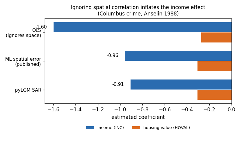
Fit the obvious regression and you get a large negative income coefficient:

CRIME = 68.62 − 1.597 · INC − 0.274 · HOVAL

But neighbourhoods are not independent draws. Crime spills across boundaries, so the residuals are spatially correlated, and OLS — which assumes they are not — attributes to income variation that is really shared local structure. The coefficient is biased, and its standard error is optimistic.

The model

pyLGM's SAR effect puts a spatial-autoregressive field on the latent scale,

\[ Q = \tau\,(I - \rho W)^\top (I - \rho W), \]

which is the spatial error model structure: \(y = X\beta + x\) with \((I - \rho W)x = \varepsilon\). The field absorbs the shared local structure so that \(\beta\) is left carrying only what income and housing value actually explain.

import json
import pandas as pd
from pylgm import Fixed, Gaussian, Hyperparameter, LGM
from pylgm.effects.spec import SAR

frame = pd.read_csv("examples/columbus_spatial_econometrics/data.csv", dtype={"id": str})
graph = json.loads(open("examples/columbus_spatial_econometrics/graph.json").read())

model = LGM(
    response="CRIME",
    predictor=Fixed("1 + INC + HOVAL") + SAR(
        "nbhd", "id", graph,
        rho=Hyperparameter("nbhd.rho", initial=0.0, transform="logit"),
        precision=Hyperparameter("nbhd.precision", initial=0.01, lower=1e-6, upper=1e3),
    ),
    likelihood=Gaussian(sigma=Hyperparameter("sigma", initial=5.0, lower=1e-2, upper=1e3)),
)
result = model.fit(frame)

Note transform="logit" on rho — it is confined to \((-1, 1)\), so the default log transform would reject an initial value of 0.0. See empirical Bayes.

The result

model	const	INC	HOVAL	ρ / λ
published OLS	68.619	−1.5973	−0.2739	—
OLS, recomputed here	68.619	−1.5973	−0.2739	—
published ML spatial error	60.279	−0.9573	−0.3046	0.5468
pyLGM SAR	59.543	−0.9057	−0.3058	0.5946

Two things are being checked here, and they are different.

The OLS row matching the published values exactly is the load-bearing one. It verifies the data, the contiguity graph, and the specification — independent of anything pyLGM does. If that row disagreed, nothing below it would mean anything.

The SAR row landing next to the published ML spatial-error estimates is the actual claim. HOVAL comes out at −0.3058 against −0.3046; the constant at 59.5 against 60.3. And the economic conclusion reproduces: ignoring spatial correlation overstates the income effect by 1.76×.

Why the fit is not identical, and should not be

pyLGM is not re-implementing maximum likelihood. Exact agreement would be suspicious rather than reassuring. Two differences account for the spread:

• It is Bayesian. The latent field is shrunk by its prior and ρ is a posterior estimate, not an ML maximiser.
• It carries a nugget. Gaussian(sigma=...) sits alongside the spatial field, so observation noise and spatial noise compete for the same variance. The ML spatial-error model has no such term. Here the nugget is squeezed toward zero, which is why the estimates land as close as they do.

The visible consequence is ρ = 0.595 against λ = 0.547.

What the spatial term is absorbing

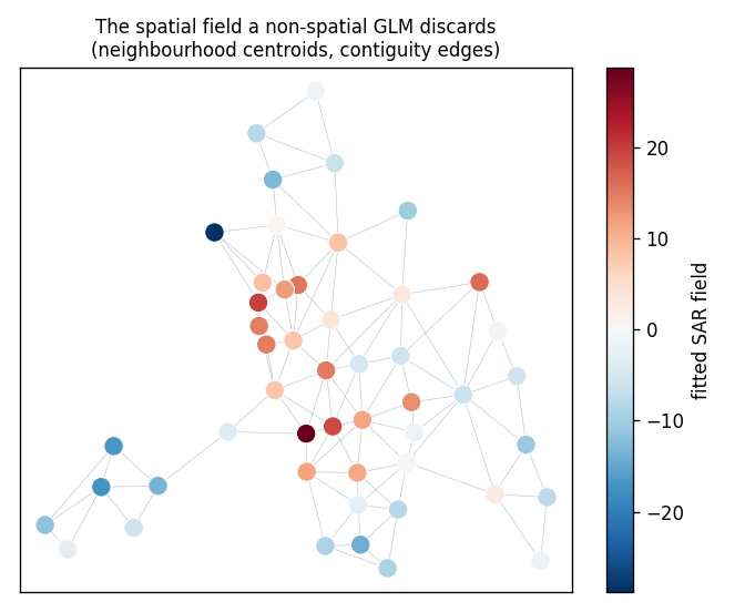
Neighbourhood centroids, contiguity edges, coloured by the fitted SAR field. The clustering is the point: neighbouring areas share elevated or depressed crime beyond what income and housing value explain. That structure is exactly what OLS folds into the income coefficient, and what the spatial field takes back out.

Takeaways

• Reproducing a published result is a stronger check than a simulation, because you did not choose the answer.
• Verify the baseline first. The exact OLS match is what licenses reading the SAR row at all.
• Expect a close match, not an identical one, when the estimator differs — and say which differences you expect to matter.