Example: spatial disease mapping vs. a standard GLM

A worked comparison on the canonical Scotland lip-cancer data (56 districts, the GeoBUGS example). For each district we have observed cases, an expected count (age-standardised), and aff — the proportion of the workforce in agriculture, fishing, and forestry, a proxy for outdoor sun exposure. Raw rates in small districts are noisy; a spatial model borrows strength from neighbours.

The full runnable script and data are in examples/disease_mapping/.

The model

observed_i ~ Poisson(mu_i)
log(mu_i)  = log(expected_i) + b0 + b1 * aff_i + s_i

where s is a Besag (ICAR) spatial effect over the district adjacency graph. The expected count enters as an offset; the covariate is an ordinary Fixed term; the spatial precision is estimated with a PC prior.

import json
import numpy as np
import pandas as pd
from pylgm import LGM, Besag, Fixed, Hyperparameter, PCPrecision, Poisson

frame = pd.read_csv("examples/disease_mapping/data.csv")
frame["area"] = frame["area"].astype(str)
frame["log_E"] = np.log(frame["expected"])
graph = json.loads(open("examples/disease_mapping/graph.json").read())

result = LGM(
    response="observed", likelihood=Poisson(), offset="log_E",
    predictor=Fixed("1 + aff") + Besag(
        "spatial", index="area", graph=graph,
        precision=Hyperparameter("spatial_prec", initial=1.0,
                                 prior=PCPrecision(upper_sd=1.0, alpha=0.01))),
).fit(frame, engine="laplace")

Spatial smoothing shrinks noisy rates

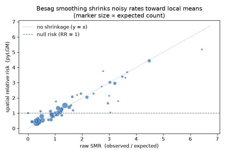
The raw standardised mortality ratio (SMR = observed / expected) swings from 0 to 6.4 across districts, much of that sampling noise in small populations. The Besag effect pulls extreme SMRs toward the level of their neighbours — the classic disease-mapping shrinkage — tightening the relative-risk spread from sd 1.31 to 1.10:

It fits far better than a covariate-only GLM

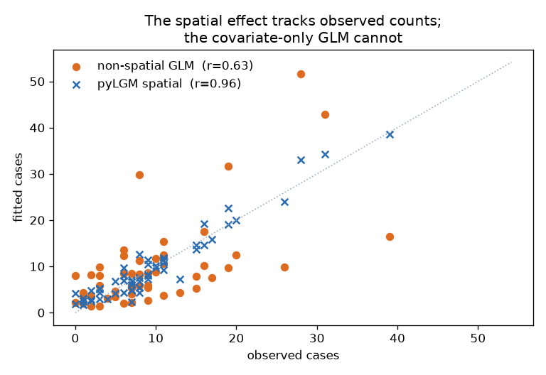
A standard non-spatial statsmodels Poisson GLM with the same offset and the same aff covariate has nowhere to absorb the district-to-district variation the covariate does not explain. Adding the spatial effect lifts the correlation between fitted and observed counts from 0.63 to 0.96:

model	corr(fitted, observed)
non-spatial Poisson GLM (aff only)	0.63
pyLGM + Besag spatial effect	0.96

The aff coefficient stays positive throughout (GLM +0.74; spatial model +0.50 ± 0.12) — once neighbouring risk is accounted for, part of what the GLM loaded onto the covariate is explained by spatial structure, a more honest attribution. The estimated spatial precision is ≈ 4.1.

Takeaways

• Spatial effects turn a covariate regression into a disease-mapping model: neighbouring areas share information, so small-area estimates stop chasing noise.
• The comparison is apples-to-apples — same likelihood, offset, and covariate — so the jump in fit (0.63 → 0.96) is purely the spatial random effect. See spatial effects for Besag, ProperCAR, and BYM2, and the theory page for why ICAR scaling matters.