Example: count regression vs. a standard GLM

A worked comparison on genuine, over-dispersed count data: the Agresti/Brockmann horseshoe crab dataset (173 female crabs). Each crab has a satellite count sat and a carapace width; bigger crabs attract more mates. We fit the mean structure, benchmark it against a standard statsmodels Poisson GLM, and show what pyLGM adds — an estimated overdispersion effect that makes the uncertainty honest.

The full runnable script and data are in examples/count_regression/.

The model

import pandas as pd
from pylgm import LGM, Fixed, Poisson

frame = pd.read_csv("examples/count_regression/data.csv")
frame["width_c"] = frame["width"] - frame["width"].mean()

poisson = LGM(
    response="sat",
    likelihood=Poisson(),
    predictor=Fixed("1 + width_c"),
).fit(frame, engine="laplace")

coeff = poisson.latent_marginals("fixed")
print(coeff.mean[1], coeff.std[1])   # width slope and its posterior sd

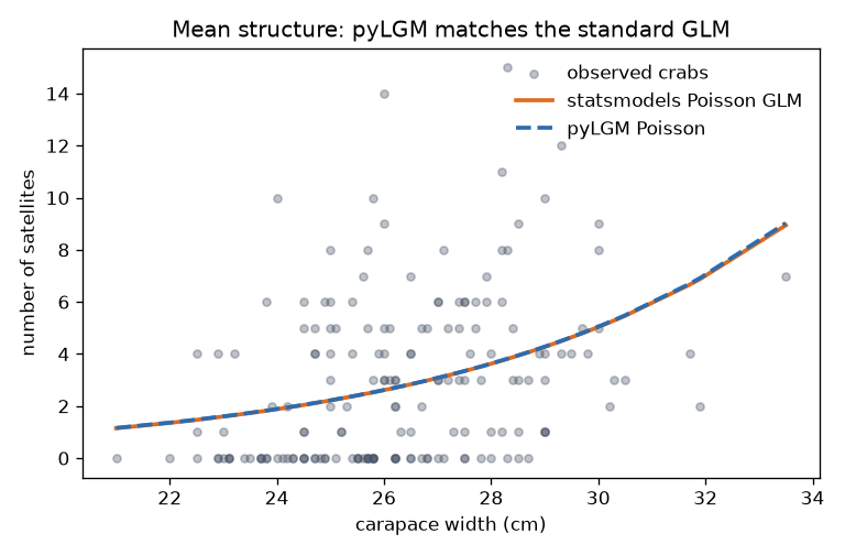
pyLGM matches the standard GLM

Fit the identical model with statsmodels and the estimates line up to three decimals — the Laplace engine reproduces the maximum-likelihood GLM when the predictor is fixed effects only:

width coefficient (log-count per cm)	estimate	std. error
statsmodels Poisson GLM	+0.164	0.020
pyLGM Poisson	+0.164	0.020

What pyLGM adds: honest overdispersion

Satellite counts are famously over-dispersed — the sample variance (9.9) is more than three times the mean (2.9), so a plain Poisson understates uncertainty. Add an IID per-crab effect with an estimated precision (a PC prior on the standard deviation) and the width CI widens to reflect the extra variability, without the point estimate drifting:

from pylgm import Hyperparameter, IID, PCPrecision

overdispersed = LGM(
    response="sat",
    likelihood=Poisson(),
    predictor=Fixed("1 + width_c") + IID(
        "od", index="crab",
        precision=Hyperparameter("od_prec", initial=1.0,
                                 prior=PCPrecision(upper_sd=2.0, alpha=0.01))),
).fit(frame, engine="laplace")

model	width coefficient	95% CI half-width
statsmodels Poisson	+0.164	±0.039
pyLGM Poisson	+0.164	±0.039
pyLGM + estimated overdispersion	+0.222	±0.090

The left panel below holds out 23 crabs and shows pyLGM predicts them identically to the standard GLM; the right panel shows the coefficient CI widening once overdispersion is modelled.

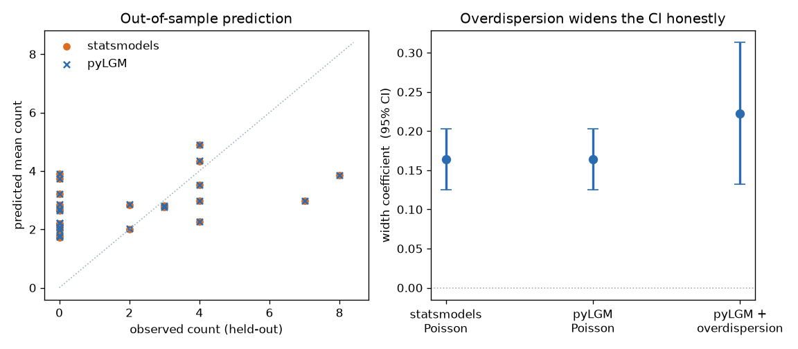
Out-of-sample RMSE is essentially identical (statsmodels 2.334, pyLGM 2.336): the mean structure is the same, so predictive accuracy is the same — pyLGM's value here is the calibrated uncertainty, not a different point forecast.

Takeaways

• On a fixed-effects GLM, pyLGM is the standard GLM — same estimates, same predictions.
• Latent effects (IID, and the spatial and temporal effects) are how you go beyond it: here, an estimated overdispersion variance the GLM has no place to put. See effects and empirical Bayes and priors.