Case study: a network that changes every year
Most spatial models fix the network once and reuse it for every period. Economic
influence does not sit still: who a region actually co-moves with shifts over a
decade. DynamicSpatialPanel
takes one network per period, so the graph itself is a time series.
The runnable script and data are in
examples/state_income_dynamic_network/.
The data and the network
Per-capita income for the 48 contiguous US states, 1997–2007, from the Bureau of Economic Analysis. The topology is real geography — state contiguity — but the edge weights are economic: neighbouring states are linked more strongly when their income levels are close.
The weight for year \(t\) is built from year \(t-1\), so the network never sees the value being modelled. That matters for the forecast at the end: the same construction works for a future period without leaking its target.
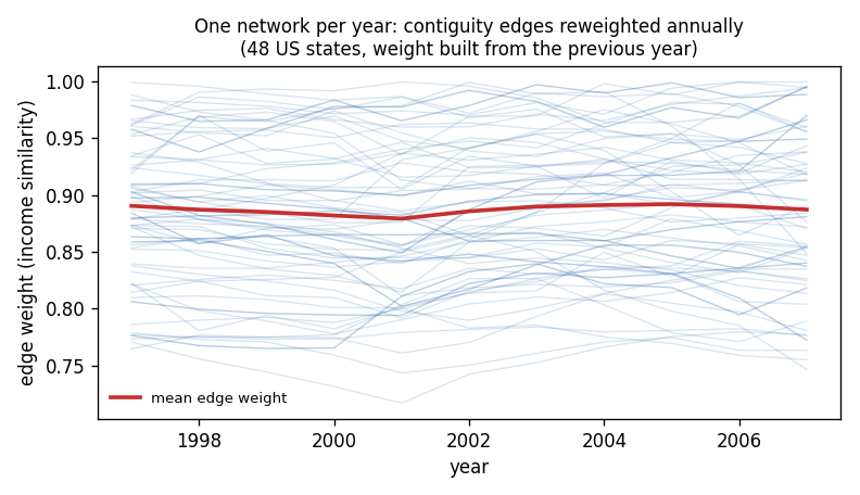
Each faint line is one contiguity edge tracked across the decade. The mean
(red) is nearly flat while individual edges move substantially — the aggregate
level of similarity is stable, but which states resemble which is not. A
static W would average that away.
The model
from pylgm import Fixed, Gaussian, Hyperparameter, LGM
from pylgm.effects.spec import DynamicSpatialPanel

effect = DynamicSpatialPanel(
    "dyn", "state", "year", graphs,          # graphs = {year: weighted_graph}
    rho=Hyperparameter("dyn.rho", initial=0.0, transform="logit"),
    gamma=Hyperparameter("dyn.gamma", initial=0.9, transform="identity",
                         lower=-2.0, upper=2.0),
    eta=Hyperparameter("dyn.eta", initial=0.0, transform="identity",
                       lower=-2.0, upper=2.0),
    precision=Hyperparameter("dyn.precision", initial=100.0, lower=1e-2, upper=1e7),
)
result = LGM(response="loginc", predictor=Fixed("1") + effect,
             likelihood=Gaussian(sigma=0.02)).fit(frame)
gamma and eta take transform="identity": unlike rho they are not
confined to \((-1, 1)\), so they live on the real line.
Three coefficients a static model conflates
rho   (neighbour spillover, same year) = +0.6393
gamma (own persistence, one year back) = +1.0052
eta   (neighbour spillover, lagged)    = −0.5960
- ρ — how much of a state's position is explained by its neighbours' this year.
- γ — how much carries over from its own last year. At ≈ 1 this is a near-unit root: log income is close to a random walk.
- η — how much of last year's neighbours reaches a state this year.
ρ > 0 with η < 0 is the familiar spatial error-correction shape: strong contemporaneous co-movement with neighbours, partly unwound the year after. A model with a single spatial parameter cannot express that at all — it has to average the two into one number.
Where the structure earns its keep
Panels have holes: late revisions, small units, series that start later. Knock out 20% of the cells and ask each method to restore them.
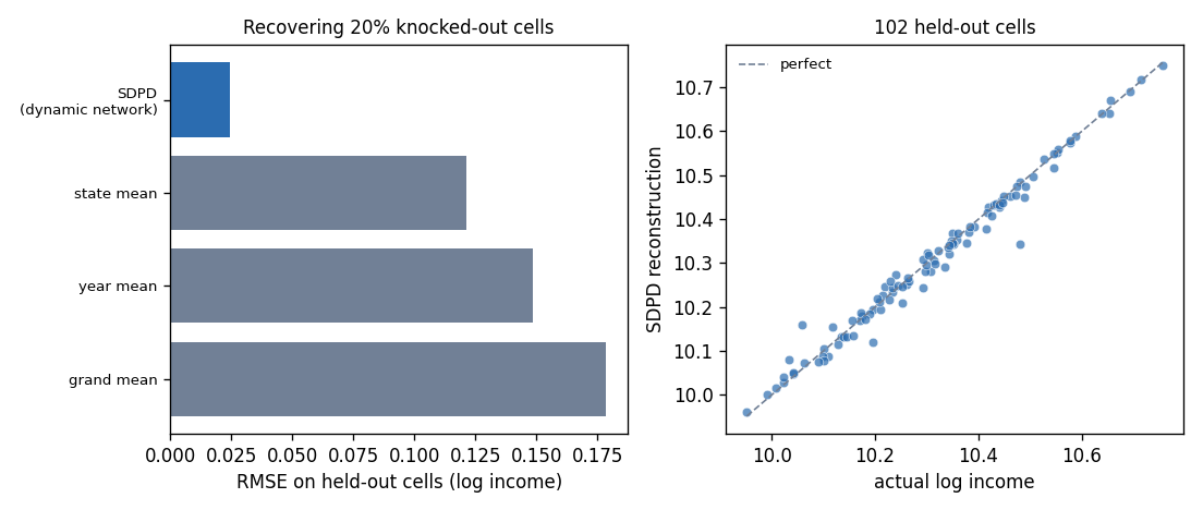
| method | RMSE ↓ (log income) |
|---|---|
DynamicSpatialPanel |
0.0246 |
| state mean | 0.1214 |
| year mean | 0.1484 |
| grand mean | 0.1786 |
About 5× closer than the obvious baselines, because a missing cell is reconstructed from both its own history and its neighbours' current values — the two axes the baselines each use only one of.
Mechanically this is the ordinary NaN-response
workflow: held-out rows keep their latent
cell and contribute no likelihood, and the SDPD precision couples that cell to
its neighbours in space and time.
Where it does not win
The example also forecasts 2008–09 and reports the honest answer:
| year | SDPD | last value |
|---|---|---|
| 2008 | 0.0397 | 0.0291 |
| 2009 | 0.1242 | 0.0255 |
A last-value benchmark wins. That is not a defect, and it follows directly from γ ≈ 1.005: for a random walk the last observed value is the optimal forecast, and no amount of structure beats it at its own game.
The useful reading is that these two results are about different questions. Filling a gap is an interpolation problem, where knowing the neighbours helps a great deal. Forecasting a near-unit-root series is an extrapolation problem, where there is little to know. A model that is good at one is not automatically good at the other, and a page that reported only the flattering number would be worth less than one you can check.
The forecast helper returns the latent field
from pylgm import forecast_dynamic_spatial_panel

forecast = forecast_dynamic_spatial_panel(result, effect, {"2008": w_2008})
beta = dict(zip(result.labels, result.mean))
forecast["predicted"] = forecast["latent_mean"] + beta["fixed:Intercept"]
latent_mean / latent_variance are the SDPD field alone — the fixed effects
are excluded, because future covariate values are an input the helper is not
given. Add them yourself before comparing with observations.
Cost
SDPD is the most expensive effect in the library: the block-bidiagonal operator
is rebuilt at every hyperparameter evaluation, and cost grows superlinearly in
units × periods (481 cells ≈ 6s, 961 cells ≈ 72s with two estimated
coefficients). Fix the coefficients you do not need estimated.
Takeaways
- A time-varying
Wis worth it when who resembles whom moves, even if the aggregate level of connection does not. - Splitting ρ / γ / η separates contemporaneous spillover, persistence and diffusion, which a single spatial parameter blends.
- Structure helps most where you are interpolating within the panel, least where you are extrapolating a random walk.